
dmrfit estimates discrete Markov Random Fields, both Ising models (Ising, 1925) and Ordinal Markov Random Fields (Marsman et al., 2025), through the pseudo-likelihood. It offers a frequentist route, with point estimates from a trust region algorithm and robust standard errors, and a Bayesian route, in which the pseudo-posterior is corrected with coordinate rescaling (CoRe; Arena and Marsman, 2026). Point estimation supports both full network estimation, where all edges are included, and constrained network estimation, where only a specified subset of edges is considered.
Main functionalities
dmrfit(): point estimation and Bayes factors - Maximum pseudo-likelihood estimation, or maximum a posteriori estimation with with_prior = TRUE (Beta-Prime prior on the thresholds, Cauchy prior on the pairwise interactions), through a trust region algorithm (Fletcher, 1987; Nocedal and Wright, 1999). - Robust standard errors from the Godambe-Huber-White (GHW, or sandwich) estimator, with Wald intervals, and with lrt_intervals = TRUE profile likelihood-ratio intervals adjusted for the pseudo-likelihood (Geys et al., 1999; Pace et al., 2011), which can be asymmetric when the sample size is small relative to the number of parameters. confint() returns either, and summary() prints them next to each other. - Constrained estimation with structure, a P x P adjacency matrix of the edges to include. - Savage-Dickey Bayes factors for each pairwise interaction with savage_dickey = TRUE, computed by sampling importance resampling from the coordinate-rescaled pseudo-posterior (Skare et al., 2003). - Gradient, Hessian and pseudo-likelihood evaluations parallelized over ncores, with the same results for any number of cores.
dmrfit_bayes(): posterior sampling - Draws from the coordinate-rescaled pseudo-posterior (method = "core", default; Arena and Marsman, 2026), which corrects the underestimated posterior variability of the pseudo-likelihood. All methods use the Fisher adaptive Metropolis-adjusted Langevin algorithm (FisherMALA; Titsias, 2024). - The pseudo-posterior is rescaled to the GHW covariance (scale = "ghw", default), or to the inverse of a Monte Carlo estimate of the Hessian of the full log-posterior, at the pseudo-posterior mode (scale = "mch") or at the Robbins-Monro estimate of the full-posterior mode (scale = "rm"). - method = "adacore" adapts the rescaling during burn-in; method = "exact" samples the full-likelihood posterior for small networks, with the normalizing constant computed by enumeration; method = "dmh" samples it with the double Metropolis-Hastings algorithm (Liang, 2010), which is much slower. - Posterior summaries (means, standard deviations, 95% credible intervals) and Savage-Dickey Bayes factors for each pairwise interaction, computed from the posterior draws; highest posterior density intervals with confint().
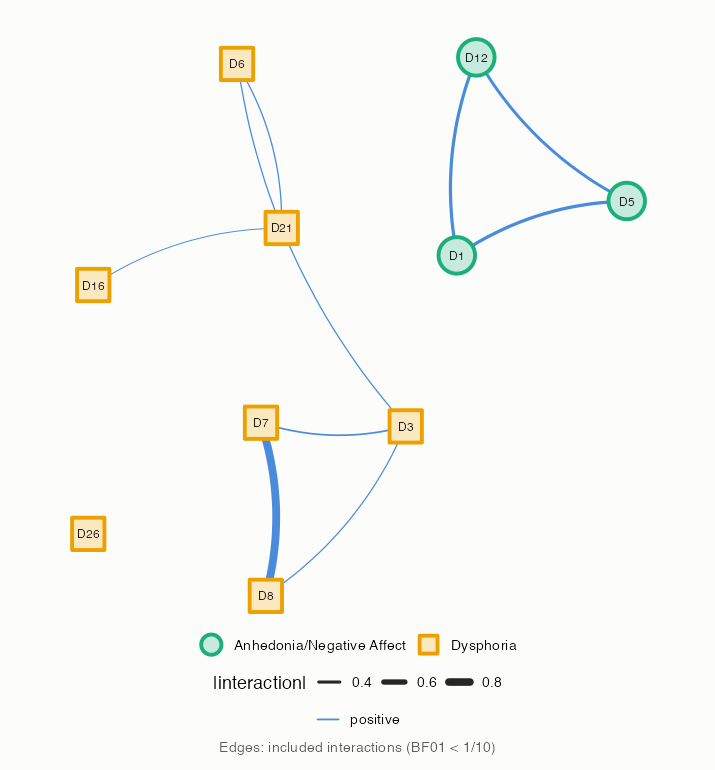
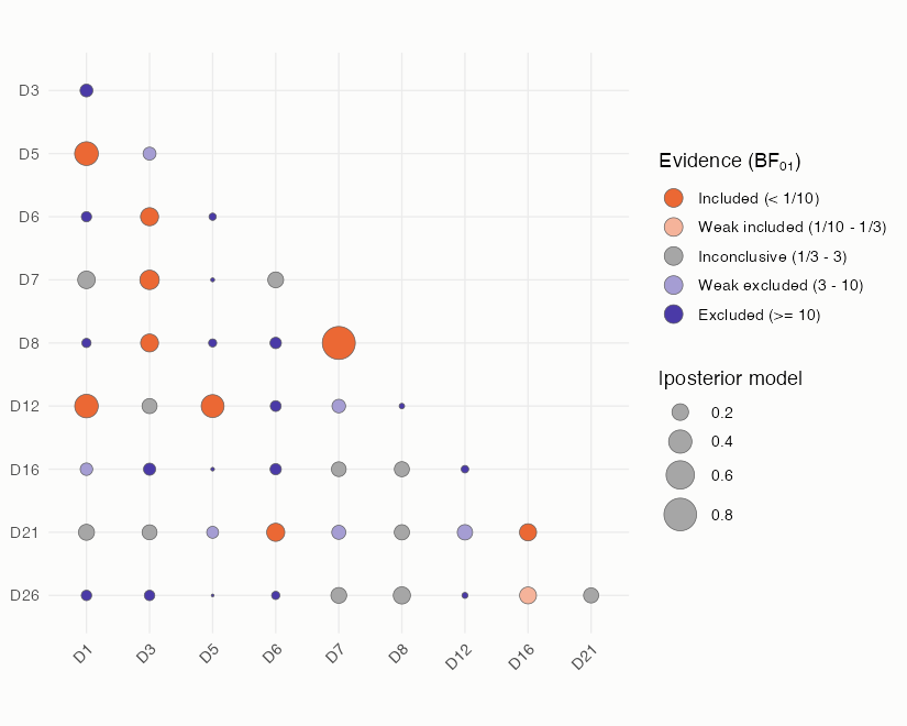
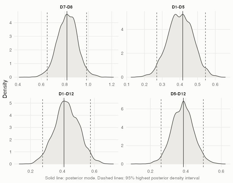
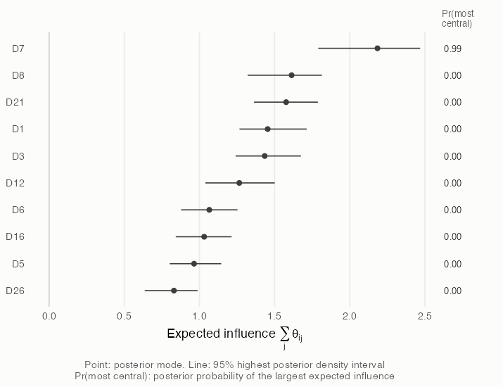
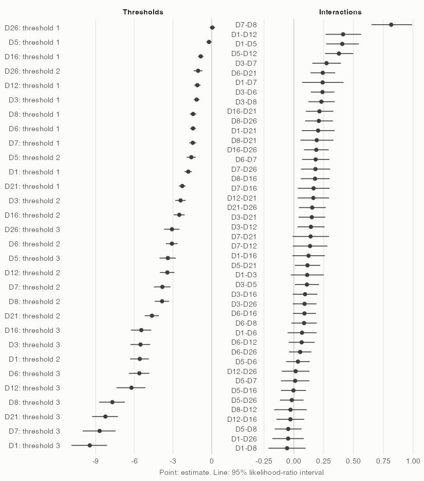
plot(): plots of both fit objects, made with ggplot2 - type = "network": the network of the included edges (Savage-Dickey Bayes factor BF01 < 1/10), with the edge width and color given by the size and sign of the interaction, and optional node groups. - type = "bf": the evidence for every edge, from excluded to included, with the size of the interaction. - type = "trace" and type = "density": the posterior draws of selected parameters, with highest posterior density intervals. - type = "intervals": the estimates and intervals of the thresholds and interactions. - type = "centrality": the expected influence of every variable, and its posterior probability of being the most central. - show_comments = FALSE leaves out the explanation below the plot, for instance when it goes into the caption of a figure in a paper.
Both fitting functions return objects with print(), summary(), confint() and plot() methods.
Installation
Install the development version from GitHub:
remotes::install_github("jupepis/dmrfit") # install package via remotes

library(dmrfit) # load the package
Example
library(dmrfit)

# RADS-2 responses of 917 adolescents (25 items, 4 ordered categories). Here the 10 items of two clusters
data(rads2)
clusters <- attr(rads2, "clusters")
items <- names(clusters)[clusters %in% c("Dysphoria", "Anhedonia/Negative Affect")]

# Point estimates, GHW standard errors, likelihood-ratio intervals and Savage-Dickey Bayes factors
fit <- dmrfit(rads2[, items], with_prior = TRUE, savage_dickey = TRUE, lrt_intervals = TRUE)
summary(fit)
confint(fit)

# Posterior sampling from the coordinate-rescaled pseudo-posterior
fit_bayes <- dmrfit_bayes(rads2[, items], nsim = 5000, burnin = 1000)
summary(fit_bayes)
The example uses rads2, data from Ramos-Vera et al. (2023) distributed under the CC BY 4.0 license (see ?rads2).
Plots
plot(fit_bayes, groups = clusters[items])  # network of the included edges, nodes grouped by cluster
plot(fit_bayes, type = "bf")               # evidence for every edge
plot(fit_bayes, type = "density")     # posterior densities of the four largest interactions
plot(fit_bayes, type = "centrality")  # expected influence of every item
plot(fit, type = "intervals") # estimates and likelihood-ratio intervals
Any issues with the package?
Should you encounter errors while using the package, or for reporting any kind of malfunction of the package, you can open an issue in here.
When opening an issue, please, use a descriptive title that clearly states the issue, be as thorough as possible when describing the issue, provide code snippets that can reproduce the issue.
References
- Arena, G. and Marsman, M. (2026). Bayesian inference for discrete Markov random fields through coordinate rescaling. arXiv preprint. https://doi.org/10.48550/arXiv.2601.17205
- Ising, E. (1925). Beitrag zur theorie des ferromagnetismus. Zeitschrift für Physik, 31(1):253–258.
- Fletcher, R. (1987). Practical Methods of Optimization. 2nd ed. Chichester: Wiley.
- Nocedal, J. and Wright, S.J. (1999). Numerical Optimization. New York: Springer.
- Geys, H., Molenberghs, G., and Ryan, L. M. (1999). Pseudolikelihood modeling of multivariate outcomes in developmental toxicology. Journal of the American Statistical Association, 94(447):734–745. https://doi.org/10.1080/01621459.1999.10474176
- Pace, L., Salvan, A., and Sartori, N. (2011). Adjusting composite likelihood ratio statistics. Statistica Sinica, 21(1):129–148.
- Liang, F. (2010). A double Metropolis-Hastings sampler for spatial models with intractable normalizing constants. Journal of Statistical Computation and Simulation, 80(9):1007–1022.
- Marsman, M., van den Bergh, D., and Haslbeck, J. M. B. (2025). Bayesian analysis of the ordinal Markov random field. Psychometrika, 90:146–182.
- Ramos-Vera, C., Quispe Callo, G., Basauri Delgado, M., Vallejos Saldarriaga, J., and Saintila, J. (2023). Factorial and network structure of the Reynolds Adolescent Depression Scale (RADS-2) in Peruvian adolescents. PLOS ONE, 18(5):e0286081.
- Skare, Ø., Bølviken, E., and Holden, L. (2003). Improved sampling-importance resampling and reduced bias importance sampling. Scandinavian Journal of Statistics, 30(4):719–737.
- Titsias, M. K. (2024). Optimal preconditioning and Fisher adaptive Langevin sampling. In Proceedings of the 37th International Conference on Neural Information Processing Systems (NIPS ’23). Red Hook, NY, USA: Curran Associates.



