Analyzing a psychological network with dmrfit • dmrfit

This vignette illustrates a complete network analysis with dmrfit. It covers point estimation with confidence intervals, the evidence for each edge, Bayesian estimation, centrality, and the choice between the sampling methods. Each section first describes how to run the analysis and interpret its output. The paragraphs titled Details explain the methods and can be skipped on a first reading. The notation follows Arena and Marsman (2026).

Discrete Markov random fields and the pseudo-likelihood

A discrete Markov random field models the conditional dependencies between discrete random variables, such as the items of a questionnaire, as a network: two variables are connected when they are dependent given all the other variables. Let $\mathbf{X} = (\mathbf{X}_1, \ldots, \mathbf{X}_n)$ denote the observed data for $n$ observations on $p$ ordinal variables, where each variable takes one of the categories $0, 1, \ldots, m$ , and let $\mathbf{X}_{\nu} = (X_{\nu 1}, \ldots, X_{\nu p})$ denote the $\nu$ -th observation. The ordinal Markov random field (OMRF) is defined by the parameter vector $\boldsymbol{\eta} = (\boldsymbol{\mu}, \boldsymbol{\theta})$ , which comprises the threshold parameters $\mu_{ih}$ , the tendency of variable $i$ to take the non-baseline category $h = 1, \ldots, m$ that is not explained by its interactions with the other variables, and the interaction parameters $\theta_{ij}$ , the pairwise conditional dependency between variables $i$ and $j$ . An interaction $\theta_{ij} = 0$ means that variables $i$ and $j$ are conditionally independent, that is, there is no edge between them. When the variables are binary, the OMRF reduces to the Ising model.

The full likelihood of the OMRF contains a normalizing constant that sums over all $(m + 1)^p$ possible response patterns, which is infeasible beyond a few variables. dmrfit uses the pseudo-likelihood instead, the product of the conditional distributions of each variable given the remaining variables, $\tilde{f}(\mathbf{X}; \boldsymbol{\eta}) = \prod_{\nu=1}^{n} \prod_{i=1}^{p} f\left(X_{\nu i} \mid \mathbf{X}_{\nu(-i)}, \boldsymbol{\eta}\right), \qquad f\left(X_{\nu i} = h \mid \mathbf{X}_{\nu(-i)}, \boldsymbol{\eta}\right) = \frac{\exp\left(\mu_{ih} + h \sum_{j \neq i} \theta_{ij} X_{\nu j}\right)} {1 + \sum_{k=1}^{m} \exp\left(\mu_{ik} + k \sum_{j \neq i} \theta_{ij} X_{\nu j}\right)},$ with $\mu_{i0} = 0$ , whose normalizing constants are computationally tractable. Combined with a prior $\pi(\boldsymbol{\eta})$ , it defines the pseudo-posterior $\tilde{\pi}(\boldsymbol{\eta} \mid \mathbf{X}) \propto \tilde{f}(\mathbf{X}; \boldsymbol{\eta})\, \pi(\boldsymbol{\eta})$ . The pseudo-likelihood estimates are consistent, but the curvature of the pseudo-likelihood overstates the information in the data: used naively, it underestimates the variability of the estimates and the posterior variance. The package corrects this underestimation in two ways.

dmrfit() estimates the parameters by maximizing the pseudo-likelihood (or the pseudo-posterior), with robust standard errors, confidence intervals and Bayes factors for the edges.
dmrfit_bayes() samples from the pseudo-posterior rescaled to the scale of the full posterior (coordinate rescaling, CoRe, Arena and Marsman, 2026).

library(dmrfit)

The data

rads2 contains the responses of 917 adolescents from Lima (Peru) to the 25 items of the four-factor version of the Reynolds Adolescent Depression Scale (RADS-2), each answered on a four-point scale (Ramos-Vera et al., 2023). The positively worded items were reverse-coded, so that higher values mean more symptoms for every item. The items belong to four clusters, stored with the data. Here we use the 10 items of two clusters, dysphoria and anhedonia/negative affect, with $p = 10$ variables, $m + 1 = 4$ categories and $n = 917$ observations.

data(rads2)
clusters <- attr(rads2, "clusters")
items <- names(clusters)[clusters %in% c("Dysphoria", "Anhedonia/Negative Affect")]
X <- rads2[, items]
clusters[items]
#>                          D1                          D3 
#> "Anhedonia/Negative Affect"                 "Dysphoria" 
#>                          D5                          D6 
#> "Anhedonia/Negative Affect"                 "Dysphoria" 
#>                          D7                          D8 
#>                 "Dysphoria"                 "Dysphoria" 
#>                         D12                         D16 
#> "Anhedonia/Negative Affect"                 "Dysphoria" 
#>                         D21                         D26 
#>                 "Dysphoria"                 "Dysphoria"

The response frequencies show that the highest category is rarely chosen for some items. This matters below, because a threshold of a rare category is estimated from few observations.

sapply(X, function(item) table(factor(item, levels = 1:4)))
#>    D1  D3  D5  D6  D7  D8 D12 D16 D21 D26
#> 1 500 275 257 417 282 323 384 325 495 177
#> 2 325 231 348 243 265 275 331 324 208 339
#> 3  66 295 200 175 281 219 137 209 151 275
#> 4  26 116 112  82  89 100  65  59  63 126

Point estimation and confidence intervals

dmrfit() estimates the thresholds and interactions. With with_prior = TRUE it maximizes the pseudo-posterior, which gives the maximum a posteriori (MAP) estimate, with beta-prime priors on the exponentiated thresholds, $\exp(\mu_{ih}) \sim \text{Beta-Prime}(0.5, 0.5)$ , and Cauchy priors on the interactions, $\theta_{ij} \sim \text{Cauchy}(0, 2.5)$ . Without the prior it gives the maximum pseudo-likelihood estimate (MPLE). lrt_intervals = TRUE adds likelihood-ratio intervals for all parameters, and savage_dickey = TRUE the Bayes factors of the next section.

fit <- dmrfit(X, with_prior = TRUE, savage_dickey = TRUE, lrt_intervals = TRUE)

In the output, mu[i,h] is the threshold $\mu_{ih}$ and theta[i,j] the interaction $\theta_{ij}$ , with the variables numbered in the column order of the data. summary() prints the estimates with their standard errors, and the Wald and likelihood-ratio intervals next to each other.

summary(fit)
#> 
#> Call:
#> dmrfit(data = X, with_prior = TRUE, savage_dickey = TRUE, lrt_intervals = TRUE)
#> 
#> Discrete Markov Random Field
#> Estimation method: maximum pseudo-likelihood (with prior)
#> Nodes: 10  Observations: 917  Free parameters: 75 
#> Standard errors: Godambe-Huber-White (GHW) estimator
#> ------------------------------------------------------------ 
#> 
#> Thresholds:
#>          Post.Mode   Post.SD  z value  Pr(>|z|)
#> mu[1,1]  -1.820877  0.144418 -12.6084 < 2.2e-16
#> mu[1,2]  -5.576649  0.370759 -15.0412 < 2.2e-16
#> mu[1,3]  -9.452950  0.705495 -13.3990 < 2.2e-16
#> mu[2,1]  -1.169270  0.115919 -10.0870 < 2.2e-16
#> mu[2,2]  -2.417688  0.205029 -11.7920 < 2.2e-16
#> mu[2,3]  -5.524127  0.387496 -14.2560 < 2.2e-16
#> mu[3,1]  -0.209862  0.105177  -1.9953   0.04601
#> mu[3,2]  -1.582957  0.180676  -8.7613 < 2.2e-16
#> mu[3,3]  -3.399964  0.323605 -10.5065 < 2.2e-16
#> mu[4,1]  -1.451465  0.114853 -12.6376 < 2.2e-16
#> mu[4,2]  -3.087075  0.231522 -13.3338 < 2.2e-16
#> mu[4,3]  -5.610251  0.404348 -13.8748 < 2.2e-16
#> mu[5,1]  -1.468367  0.140364 -10.4611 < 2.2e-16
#> mu[5,2]  -3.827827  0.327542 -11.6865 < 2.2e-16
#> mu[5,3]  -8.693257  0.650305 -13.3680 < 2.2e-16
#> mu[6,1]  -1.445533  0.129159 -11.1918 < 2.2e-16
#> mu[6,2]  -3.850868  0.282119 -13.6498 < 2.2e-16
#> mu[6,3]  -7.703633  0.506745 -15.2022 < 2.2e-16
#> mu[7,1]  -1.112222  0.128882  -8.6298 < 2.2e-16
#> mu[7,2]  -3.438122  0.283897 -12.1105 < 2.2e-16
#> mu[7,3]  -6.222909  0.568813 -10.9402 < 2.2e-16
#> mu[8,1]  -0.850789  0.108832  -7.8175 5.389e-15
#> mu[8,2]  -2.513389  0.216437 -11.6125 < 2.2e-16
#> mu[8,3]  -5.457662  0.402758 -13.5507 < 2.2e-16
#> mu[9,1]  -2.282995  0.131021 -17.4247 < 2.2e-16
#> mu[9,2]  -4.633978  0.279444 -16.5829 < 2.2e-16
#> mu[9,3]  -8.242312  0.510441 -16.1474 < 2.2e-16
#> mu[10,1]  0.045836  0.107724   0.4255   0.67048
#> mu[10,2] -1.056172  0.173051  -6.1032 1.039e-09
#> mu[10,3] -3.082789  0.305565 -10.0888 < 2.2e-16
#> 
#> Pairwise interactions:
#>              Post.Mode    Post.SD z value  Pr(>|z|)    
#> theta[2,1]   0.1121620  0.0703940  1.5933 0.1110827    
#> theta[3,1]   0.4062825  0.0694625  5.8490 4.947e-09 ***
#> theta[4,1]   0.0689947  0.0617306  1.1177 0.2637062    
#> theta[5,1]   0.2416338  0.0884372  2.7323 0.0062900 ** 
#> theta[6,1]  -0.0561661  0.0794795 -0.7067 0.4797695    
#> theta[7,1]   0.4131106  0.0758050  5.4496 5.047e-08 ***
#> theta[8,1]   0.1234728  0.0690276  1.7887 0.0736560 .  
#> theta[9,1]   0.2035943  0.0701258  2.9033 0.0036929 ** 
#> theta[10,1] -0.0476660  0.0672855 -0.7084 0.4786879    
#> theta[3,2]   0.1099157  0.0517141  2.1255 0.0335490 *  
#> theta[4,2]   0.2402308  0.0504967  4.7574 1.961e-06 ***
#> theta[5,2]   0.2744462  0.0614688  4.4648 8.014e-06 ***
#> theta[6,2]   0.2313118  0.0564412  4.0983 4.162e-05 ***
#> theta[7,2]   0.1433946  0.0575102  2.4934 0.0126535 *  
#> theta[8,2]   0.0939737  0.0524526  1.7916 0.0731982 .  
#> theta[9,2]   0.1510427  0.0572081  2.6402 0.0082850 ** 
#> theta[10,2]  0.0902188  0.0507052  1.7793 0.0751938 .  
#> theta[4,3]   0.0343960  0.0504221  0.6822 0.4951364    
#> theta[5,3]   0.0113068  0.0603851  0.1872 0.8514689    
#> theta[6,3]  -0.0468243  0.0572661 -0.8177 0.4135508    
#> theta[7,3]   0.3783185  0.0600302  6.3021 2.936e-10 ***
#> theta[8,3]  -0.0029214  0.0531458 -0.0550 0.9561629    
#> theta[9,3]   0.1144986  0.0540580  2.1181 0.0341691 *  
#> theta[10,3] -0.0168471  0.0506416 -0.3327 0.7393810    
#> theta[5,4]   0.1831356  0.0584058  3.1356 0.0017152 ** 
#> theta[6,4]   0.0861031  0.0541438  1.5903 0.1117747    
#> theta[7,4]   0.0657230  0.0555872  1.1823 0.2370703    
#> theta[8,4]   0.0894205  0.0495450  1.8048 0.0711011 .  
#> theta[9,4]   0.2424225  0.0527873  4.5924 4.381e-06 ***
#> theta[10,4]  0.0534099  0.0480940  1.1105 0.2667697    
#> theta[6,5]   0.8163969  0.0866513  9.4216 < 2.2e-16 ***
#> theta[7,5]   0.1360569  0.0740861  1.8365 0.0662881 .  
#> theta[8,5]   0.1658596  0.0679567  2.4407 0.0146602 *  
#> theta[9,5]   0.1407857  0.0779097  1.8070 0.0707566 .  
#> theta[10,5]  0.1813855  0.0623835  2.9076 0.0036423 ** 
#> theta[7,6]  -0.0278154  0.0694366 -0.4006 0.6887246    
#> theta[8,6]   0.1779921  0.0614563  2.8962 0.0037766 ** 
#> theta[9,6]   0.1920124  0.0705658  2.7210 0.0065076 ** 
#> theta[10,6]  0.2100408  0.0593717  3.5377 0.0004036 ***
#> theta[8,7]  -0.0286764  0.0594765 -0.4821 0.6297012    
#> theta[9,7]   0.1635554  0.0672080  2.4336 0.0149508 *  
#> theta[10,7]  0.0152829  0.0590018  0.2590 0.7956162    
#> theta[9,8]   0.2149666  0.0587718  3.6576 0.0002545 ***
#> theta[10,8]  0.1885638  0.0529913  3.5584 0.0003731 ***
#> theta[10,9]  0.1542764  0.0574723  2.6844 0.0072668 ** 
#> ---
#> Signif. codes:  0 '***' 0.001 '**' 0.01 '*' 0.05 '.' 0.1 ' ' 1
#> 
#> Intervals (95%): Wald (GHW standard errors) and likelihood-ratio
#>             Wald lower Wald upper LRT lower LRT upper
#> mu[1,1]        -2.1039    -1.5378   -2.1084   -1.5420
#> mu[1,2]        -6.3033    -4.8500   -6.3232   -4.8697
#> mu[1,3]       -10.8357    -8.0702  -10.8810   -8.1158
#> mu[2,1]        -1.3965    -0.9421   -1.3976   -0.9430
#> mu[2,2]        -2.8195    -2.0158   -2.8260   -2.0219
#> mu[2,3]        -6.2836    -4.7646   -6.3009   -4.7818
#> mu[3,1]        -0.4160    -0.0037   -0.4156   -0.0031
#> mu[3,2]        -1.9371    -1.2288   -1.9406   -1.2319
#> mu[3,3]        -4.0342    -2.7657   -4.0485   -2.7794
#> mu[4,1]        -1.6766    -1.2264   -1.6787   -1.2282
#> mu[4,2]        -3.5409    -2.6333   -3.5508   -2.6428
#> mu[4,3]        -6.4028    -4.8177   -6.4247   -4.8395
#> mu[5,1]        -1.7435    -1.1933   -1.7456   -1.1951
#> mu[5,2]        -4.4698    -3.1859   -4.4842   -3.1999
#> mu[5,3]        -9.9678    -7.4187  -10.0023   -7.4533
#> mu[6,1]        -1.6987    -1.1924   -1.7008   -1.1943
#> mu[6,2]        -4.4038    -3.2979   -4.4153   -3.3092
#> mu[6,3]        -8.6968    -6.7104   -8.7206   -6.7343
#> mu[7,1]        -1.3648    -0.8596   -1.3668   -0.8614
#> mu[7,2]        -3.9945    -2.8817   -4.0077   -2.8943
#> mu[7,3]        -7.3378    -5.1081   -7.3762   -5.1463
#> mu[8,1]        -1.0641    -0.6375   -1.0649   -0.6381
#> mu[8,2]        -2.9376    -2.0892   -2.9453   -2.0964
#> mu[8,3]        -6.2471    -4.6683   -6.2679   -4.6889
#> mu[9,1]        -2.5398    -2.0262   -2.5436   -2.0298
#> mu[9,2]        -5.1817    -4.0863   -5.1954   -4.0999
#> mu[9,3]        -9.2428    -7.2419   -9.2697   -7.2691
#> mu[10,1]       -0.1653     0.2570   -0.1640    0.2585
#> mu[10,2]       -1.3953    -0.7170   -1.3974   -0.7186
#> mu[10,3]       -3.6817    -2.4839   -3.6938   -2.4955
#> theta[2,1]     -0.0258     0.2501   -0.0250    0.2512
#> theta[3,1]      0.2701     0.5424    0.2724    0.5450
#> theta[4,1]     -0.0520     0.1900   -0.0518    0.1904
#> theta[5,1]      0.0683     0.4150    0.0699    0.4170
#> theta[6,1]     -0.2119     0.0996   -0.2123    0.0996
#> theta[7,1]      0.2645     0.5617    0.2668    0.5644
#> theta[8,1]     -0.0118     0.2588   -0.0116    0.2594
#> theta[9,1]      0.0662     0.3410    0.0671    0.3424
#> theta[10,1]    -0.1795     0.0842   -0.1798    0.0842
#> theta[3,2]      0.0086     0.2113    0.0089    0.2119
#> theta[4,2]      0.1413     0.3392    0.1423    0.3404
#> theta[5,2]      0.1540     0.3949    0.1553    0.3964
#> theta[6,2]      0.1207     0.3419    0.1218    0.3432
#> theta[7,2]      0.0307     0.2561    0.0313    0.2570
#> theta[8,2]     -0.0088     0.1968   -0.0085    0.1973
#> theta[9,2]      0.0389     0.2632    0.0399    0.2644
#> theta[10,2]    -0.0092     0.1896   -0.0088    0.1901
#> theta[4,3]     -0.0644     0.1332   -0.0645    0.1333
#> theta[5,3]     -0.1070     0.1297   -0.1071    0.1298
#> theta[6,3]     -0.1591     0.0654   -0.1595    0.0652
#> theta[7,3]      0.2607     0.4960    0.2627    0.4983
#> theta[8,3]     -0.1071     0.1012   -0.1073    0.1012
#> theta[9,3]      0.0085     0.2205    0.0089    0.2211
#> theta[10,3]    -0.1161     0.0824   -0.1164    0.0824
#> theta[5,4]      0.0687     0.2976    0.0695    0.2987
#> theta[6,4]     -0.0200     0.1922   -0.0196    0.1928
#> theta[7,4]     -0.0432     0.1747   -0.0433    0.1749
#> theta[8,4]     -0.0077     0.1865   -0.0075    0.1870
#> theta[9,4]      0.1390     0.3459    0.1400    0.3472
#> theta[10,4]    -0.0409     0.1477   -0.0407    0.1480
#> theta[6,5]      0.6466     0.9862    0.6517    0.9917
#> theta[7,5]     -0.0091     0.2813   -0.0086    0.2822
#> theta[8,5]      0.0327     0.2991    0.0336    0.3003
#> theta[9,5]     -0.0119     0.2935   -0.0106    0.2952
#> theta[10,5]     0.0591     0.3037    0.0600    0.3048
#> theta[7,6]     -0.1639     0.1083   -0.1643    0.1082
#> theta[8,6]      0.0575     0.2984    0.0584    0.2996
#> theta[9,6]      0.0537     0.3303    0.0549    0.3319
#> theta[10,6]     0.0937     0.3264    0.0947    0.3277
#> theta[8,7]     -0.1452     0.0879   -0.1457    0.0877
#> theta[9,7]      0.0318     0.2953    0.0324    0.2963
#> theta[10,7]    -0.1004     0.1309   -0.1005    0.1310
#> theta[9,8]      0.0998     0.3302    0.1007    0.3314
#> theta[10,8]     0.0847     0.2924    0.0855    0.2934
#> theta[10,9]     0.0416     0.2669    0.0424    0.2680
#> 
#> Negative log pseudo-likelihood: 9654.417 
#> 
#> Savage-Dickey density ratio  [prior: Cauchy( 0 , 2.5 )]
#> H0: theta = 0 for each pairwise interaction
#> 
#>             Estimate     SE    BF_01 Pr(=0|x)
#> theta[2,1]    0.1122 0.0704    12.35   0.9251
#> theta[3,1]    0.4063 0.0695 < 0.0001 < 0.0001
#> theta[4,1]    0.0690 0.0617    24.28   0.9604
#> theta[5,1]    0.2416 0.0884   0.8117    0.448
#> theta[6,1]   -0.0562 0.0795    29.92   0.9677
#> theta[7,1]    0.4131 0.0758 < 0.0001 < 0.0001
#> theta[8,1]    0.1235 0.0690    10.83   0.9155
#> theta[9,1]    0.2036 0.0701    1.132   0.5309
#> theta[10,1]  -0.0477 0.0673    30.68   0.9684
#> theta[3,2]    0.1099 0.0517    9.208    0.902
#> theta[4,2]    0.2402 0.0505 < 0.0001 < 0.0001
#> theta[5,2]    0.2744 0.0615 < 0.0001 < 0.0001
#> theta[6,2]    0.2313 0.0564 < 0.0001 < 0.0001
#> theta[7,2]    0.1434 0.0575    1.512    0.602
#> theta[8,2]    0.0940 0.0525    12.54   0.9261
#> theta[9,2]    0.1510 0.0572    1.667    0.625
#> theta[10,2]   0.0902 0.0507    15.88   0.9408
#> theta[4,3]    0.0344 0.0504       51   0.9808
#> theta[5,3]    0.0113 0.0604    58.36   0.9832
#> theta[6,3]   -0.0468 0.0573    38.94    0.975
#> theta[7,3]    0.3783 0.0600 < 0.0001 < 0.0001
#> theta[8,3]   -0.0029 0.0531    61.41    0.984
#> theta[9,3]    0.1145 0.0541    6.342   0.8638
#> theta[10,3]  -0.0168 0.0506    60.07   0.9836
#> theta[5,4]    0.1831 0.0584   0.6128   0.3799
#> theta[6,4]    0.0861 0.0541    21.56   0.9557
#> theta[7,4]    0.0657 0.0556    26.24   0.9633
#> theta[8,4]    0.0894 0.0495    8.474   0.8944
#> theta[9,4]    0.2424 0.0528 < 0.0001 < 0.0001
#> theta[10,4]   0.0534 0.0481    41.02   0.9762
#> theta[6,5]    0.8164 0.0867 < 0.0001 < 0.0001
#> theta[7,5]    0.1361 0.0741    10.09   0.9098
#> theta[8,5]    0.1659 0.0680    1.655   0.6233
#> theta[9,5]    0.1408 0.0779     9.86   0.9079
#> theta[10,5]   0.1814 0.0624    1.816   0.6448
#> theta[7,6]   -0.0278 0.0694    46.33   0.9789
#> theta[8,6]    0.1780 0.0615    0.809   0.4472
#> theta[9,6]    0.1920 0.0706    1.017   0.5041
#> theta[10,6]   0.2100 0.0594 < 0.0001 < 0.0001
#> theta[8,7]   -0.0287 0.0595    42.37   0.9769
#> theta[9,7]    0.1636 0.0672    1.834   0.6471
#> theta[10,7]   0.0153 0.0590    45.56   0.9785
#> theta[9,8]    0.2150 0.0588  0.05081  0.04836
#> theta[10,8]   0.1886 0.0530 < 0.0001 < 0.0001
#> theta[10,9]   0.1543 0.0575    1.487   0.5979
#> 
#> '<': zero lies beyond all resampled draws, so BF_01 is only bounded (very strong evidence for an interaction).
#> 
#> SIR samples: 1000   Effective sample size of the importance sample: 2648.7 (of 10000 proposal draws)

The two kinds of intervals agree for most parameters, but not for the thresholds of the rarely chosen highest categories. For item D1, whose highest category was chosen 26 times, the likelihood-ratio interval of $\mu_{13}$ extends further below the estimate than above it, which the symmetric Wald interval cannot do:

confint(fit, parm = c("mu[1,3]", "theta[2,1]"))
#>                   2.5 %     97.5 %
#> mu[1,3]    -10.88102304 -8.1158110
#> theta[2,1]  -0.02504397  0.2512157
confint(fit, parm = c("mu[1,3]", "theta[2,1]"), method = "wald")
#>                   2.5 %     97.5 %
#> mu[1,3]    -10.83569524 -8.0702043
#> theta[2,1]  -0.02580772  0.2501316

plot(fit, type = "intervals") shows the estimates and intervals of all parameters, the thresholds and the interactions in separate panels, each sorted by estimate.

plot(fit, type = "intervals")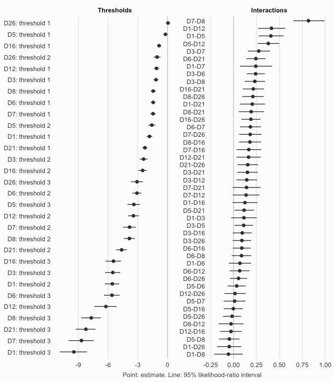

Estimates and likelihood-ratio intervals of the thresholds and interactions of the 10 items, sorted by estimate

plot of chunk intervals

When the sample is small relative to the number of parameters and the likelihood-ratio intervals are not computed, dmrfit() warns that the Wald intervals may be inaccurate:

fit_small <- dmrfit(X[1:200, ])
#> Warning in dmrfit(X[1:200, ]): The sample size (200) is small relative to the
#> number of free parameters (75): the Wald intervals assume a symmetric sampling
#> distribution and may be inaccurate. Likelihood-ratio intervals are suggested:
#> refit with lrt_intervals = TRUE (or a vector of parameter names).

Details. The standard errors come from the Godambe-Huber-White (GHW, or sandwich) covariance $\boldsymbol{\Sigma}_{\text{GHW}} = \left(-\mathbf{H}^{-1}\right) \mathbf{U} \left(-\mathbf{H}^{-1}\right),$ where $\mathbf{H}$ is the Hessian of the log pseudo-likelihood and $\mathbf{U} = \sum_{\nu=1}^{n} \mathbf{u}_{\nu} \mathbf{u}_{\nu}^{\intercal}$ the variance of the score, both evaluated at the estimate $\hat{\boldsymbol{\eta}}$ . The naive covariance $-\mathbf{H}^{-1}$ would underestimate the variability. The likelihood-ratio interval of a parameter $\eta_k$ is based on its profile: for every value of $\eta_k$ , the other parameters are set to the values that maximize the pseudo-likelihood. Because it is computed from a pseudo-likelihood, the profile likelihood-ratio statistic is not $\chi^2_1$ -distributed but $\lambda_k \chi^2_1$ -distributed, with $\lambda_k = [\boldsymbol{\Sigma}_{\text{GHW}}]_{kk} / [-\mathbf{H}^{-1}]_{kk}$ (Geys, Molenberghs and Ryan, 1999; Pace, Salvan and Sartori, 2011). The interval collects the values of $\eta_k$ for which $\frac{2}{\lambda_k} \left[\log \tilde{f}(\mathbf{X}; \hat{\boldsymbol{\eta}}) - \max_{\boldsymbol{\eta}_{-k}} \log \tilde{f}(\mathbf{X}; \eta_k, \boldsymbol{\eta}_{-k})\right] \leq \chi^2_{1, 1 - \alpha},$ with $\chi^2_{1, 1 - \alpha}$ the quantile of the $\chi^2_1$ distribution at the level of the interval. When a prior is used, the pseudo-posterior takes the place of the pseudo-likelihood, and $\lambda_k$ is computed from its curvature $-(\mathbf{H} + \mathbf{H}_{\boldsymbol{\eta}})$ , with $\mathbf{H}_{\boldsymbol{\eta}}$ the Hessian of the log prior, and from the posterior GHW covariance $\boldsymbol{\Gamma}\boldsymbol{\Gamma}^{\intercal}_{\text{GHW}} = (\boldsymbol{\Sigma}_{\text{GHW}}^{-1} - \mathbf{H}_{\boldsymbol{\eta}})^{-1}$ . The interval follows the shape of the pseudo-likelihood, so it can be asymmetric, and in large samples it agrees with the Wald interval.

A network structure can also be imposed with structure, a matrix with 1 for the edges to estimate and 0 for the edges fixed at zero. For instance, without edges between the two clusters:

S <- outer(clusters[items], clusters[items], "==") * 1
diag(S) <- 0
fit_within <- dmrfit(X, structure = S, with_prior = TRUE)
plot(fit_within, all_edges = TRUE, groups = clusters[items])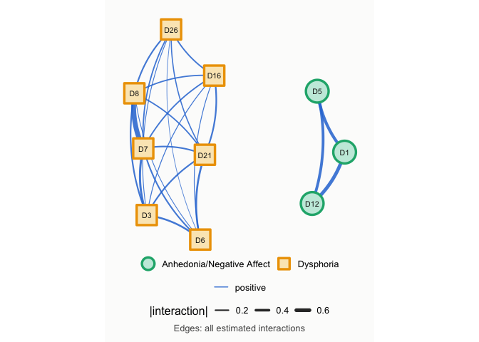

Network of the constrained fit without edges between the two clusters, with the nodes grouped by cluster

plot of chunk network-within

Is the edge there? Bayes factors

An interaction estimated close to zero does not tell whether the edge is absent or the data are not informative enough to tell. The Savage-Dickey Bayes factor $\text{BF}_{01}$ (denoted $\text{BF}_{\text{cu}}$ in Arena and Marsman, 2026) compares the hypothesis of conditional independence, $\theta_{ij} = 0$ , with the hypothesis $\theta_{ij} \neq 0$ : $\text{BF}_{01} > 1$ is evidence for conditional independence (no edge), and $\text{BF}_{01} < 1$ evidence for an interaction. The plots classify the evidence for each edge as

$\text{BF}_{01}$	Evidence
$< 1/10$	included
$1/10$ to $1/3$	weak included
$1/3$ to $3$	inconclusive
$3$ to $10$	weak excluded
$\geq 10$	excluded

evidence <- table(cut(fit$savage_dickey$bf_01, c(0, 1/10, 1/3, 3, 10, Inf), right = FALSE,
                      labels = c("included", "weak included", "inconclusive", "weak excluded", "excluded")))
evidence
#> 
#>      included weak included  inconclusive weak excluded      excluded 
#>            11             0            11             4            19

Of the 45 possible edges, 11 are included and 19 excluded, and the data leave 11 inconclusive. plot(fit, type = "bf") shows the evidence for every edge, with the size of the circle given by the size of the interaction, and the network plot draws the included edges.

plot(fit, type = "bf")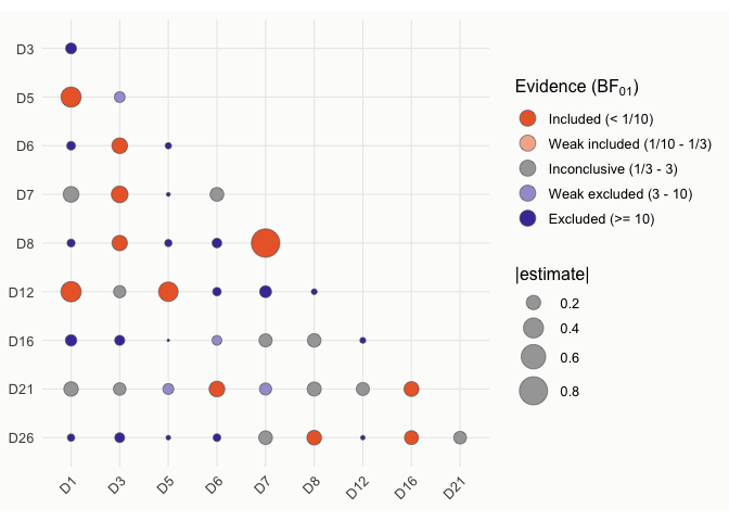

Evidence for every edge from its Savage-Dickey Bayes factor, with the size of the interaction

plot of chunk bf-network

plot(fit, groups = clusters[items])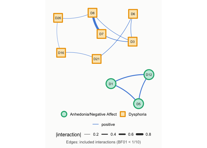

Network of the included edges, with the nodes grouped by cluster

plot of chunk bf-network

Details. The Savage-Dickey Bayes factor is the ratio of the marginal posterior and the prior density of the interaction at zero, $\text{BF}_{01} = \pi(\theta_{ij} = 0 \mid \mathbf{X}) / \pi(\theta_{ij} = 0)$ . dmrfit() estimates the posterior density from draws of the coordinate-rescaled pseudo-posterior (see the next section), obtained by sampling importance resampling (Skare et al., 2003). When zero lies beyond all draws of an interaction (10 interactions here), the density at zero cannot be estimated. The Bayes factor is then set at the floor $1/(10M)$ , with $M$ the number of resampled draws, a bound that indicates very strong evidence for an interaction, and summary() marks it with <.

Bayesian estimation with coordinate rescaling

dmrfit_bayes() samples from the posterior of the parameters. By default, it samples the coordinate-rescaled pseudo-posterior, which has the location of the pseudo-posterior and the scale of the GHW covariance.

fit_bayes <- dmrfit_bayes(X, nsim = 10000, burnin = 1000, progress = FALSE)

We first assess the convergence and mixing of the chain. The trace plot shows the draws of the interactions with the largest absolute posterior modes, which should fluctuate around a stable level, without trends. The effective sample sizes (ESS) summarize the mixing.

plot(fit_bayes, type = "trace")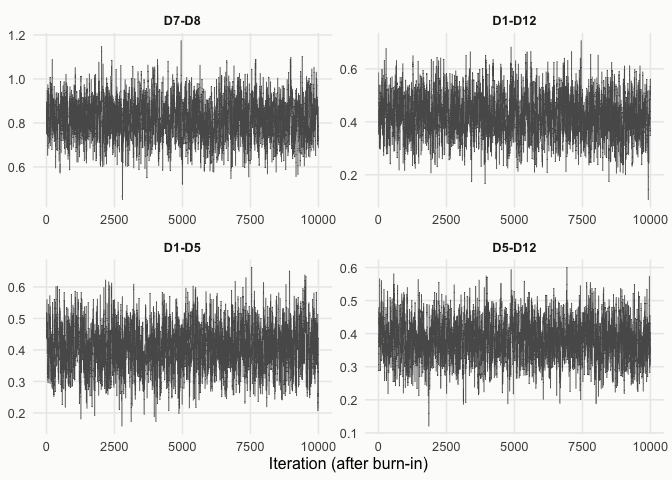

Trace plots of the posterior draws of the four interactions with the largest absolute posterior modes

plot of chunk trace

min(fit_bayes$savage_dickey$ess)  # smallest effective sample size of a parameter
#> [1] 741.6517
fit_bayes$mess                    # multivariate effective sample size of all draws
#> [1] 2006.834

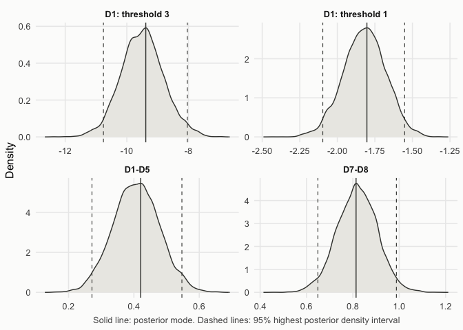
The posterior densities show the posterior mode (solid line) and the 95% highest posterior density interval (dashed lines), the shortest interval that contains 95% of the posterior.

plot(fit_bayes, type = "density", pars = c("mu[1,3]", "mu[1,1]", "theta[3,1]", "theta[6,5]"))

Posterior densities of two thresholds and two interactions, with their posterior modes and highest posterior density intervals

plot of chunk density

summary() reports the posterior summaries and the Bayes factors computed from the draws, and confint() the highest posterior density intervals. The Bayes factors from the draws and from dmrfit() agree closely: they classify 87% of the edges in the same evidence class.

summary(fit_bayes)
#> 
#> Call:
#> dmrfit_bayes(data = X, nsim = 10000, burnin = 1000, progress = FALSE)
#> 
#> Discrete Markov Random Field
#> Estimation method: Bayesian (FisherMALA), coordinate-rescaled pseudo-posterior (Godambe-Huber-White covariance) 
#> Nodes: 10  Observations: 917  Parameters: 75 
#> MCMC samples: 10000  Acceptance rate: 0.579  Elapsed: 5.5 sec
#> Multivariate effective sample size: 2006.8 
#> ------------------------------------------------------------ 
#> 
#> Thresholds:
#>          Post.Mode Post.Mean Post.SD     2.5%   97.5%
#> mu[1,1]    -1.8209   -1.8195  0.1413  -2.0957 -1.5488
#> mu[1,2]    -5.5766   -5.5764  0.3624  -6.2736 -4.8548
#> mu[1,3]    -9.4529   -9.4953  0.6911 -10.8322 -8.0860
#> mu[2,1]    -1.1693   -1.1648  0.1157  -1.3961 -0.9486
#> mu[2,2]    -2.4177   -2.4062  0.2061  -2.8224 -1.9958
#> mu[2,3]    -5.5241   -5.5083  0.3879  -6.2669 -4.7586
#> mu[3,1]    -0.2099   -0.2078  0.1063  -0.4132 -0.0033
#> mu[3,2]    -1.5830   -1.5719  0.1842  -1.9278 -1.2050
#> mu[3,3]    -3.4000   -3.3915  0.3237  -4.0296 -2.7634
#> mu[4,1]    -1.4515   -1.4448  0.1178  -1.6742 -1.2167
#> mu[4,2]    -3.0871   -3.0676  0.2371  -3.5437 -2.6209
#> mu[4,3]    -5.6103   -5.5944  0.4105  -6.4140 -4.8052
#> mu[5,1]    -1.4684   -1.4695  0.1430  -1.7454 -1.1861
#> mu[5,2]    -3.8278   -3.8291  0.3309  -4.4680 -3.1688
#> mu[5,3]    -8.6933   -8.6951  0.6522  -9.9747 -7.4016
#> mu[6,1]    -1.4455   -1.4365  0.1340  -1.6989 -1.1778
#> mu[6,2]    -3.8509   -3.8328  0.2891  -4.3973 -3.2692
#> mu[6,3]    -7.7036   -7.6765  0.5182  -8.6959 -6.6631
#> mu[7,1]    -1.1122   -1.1050  0.1290  -1.3637 -0.8641
#> mu[7,2]    -3.4381   -3.4370  0.2822  -3.9856 -2.8854
#> mu[7,3]    -6.2229   -6.2466  0.5712  -7.3548 -5.1115
#> mu[8,1]    -0.8508   -0.8460  0.1077  -1.0579 -0.6352
#> mu[8,2]    -2.5134   -2.4993  0.2163  -2.9321 -2.0811
#> mu[8,3]    -5.4577   -5.4531  0.4114  -6.2679 -4.6529
#> mu[9,1]    -2.2830   -2.2898  0.1317  -2.5436 -2.0331
#> mu[9,2]    -4.6340   -4.6481  0.2760  -5.1841 -4.0957
#> mu[9,3]    -8.2423   -8.2867  0.5058  -9.2708 -7.2805
#> mu[10,1]    0.0458    0.0569  0.1069  -0.1518  0.2675
#> mu[10,2]   -1.0562   -1.0324  0.1747  -1.3797 -0.6839
#> mu[10,3]   -3.0828   -3.0376  0.3082  -3.6558 -2.4412
#> 
#> Pairwise interactions:
#>             Post.Mode Post.Mean Post.SD    2.5%  97.5%
#> theta[2,1]     0.1122    0.1191  0.0698 -0.0163 0.2603
#> theta[3,1]     0.4063    0.4072  0.0705  0.2712 0.5467
#> theta[4,1]     0.0690    0.0715  0.0616 -0.0484 0.1937
#> theta[5,1]     0.2416    0.2470  0.0899  0.0664 0.4230
#> theta[6,1]    -0.0562   -0.0593  0.0808 -0.2188 0.0985
#> theta[7,1]     0.4131    0.4232  0.0776  0.2709 0.5757
#> theta[8,1]     0.1235    0.1219  0.0682 -0.0100 0.2562
#> theta[9,1]     0.2036    0.1995  0.0708  0.0603 0.3414
#> theta[10,1]   -0.0477   -0.0575  0.0670 -0.1883 0.0727
#> theta[3,2]     0.1099    0.1116  0.0513  0.0108 0.2135
#> theta[4,2]     0.2402    0.2405  0.0510  0.1377 0.3405
#> theta[5,2]     0.2744    0.2778  0.0618  0.1567 0.3995
#> theta[6,2]     0.2313    0.2297  0.0575  0.1168 0.3432
#> theta[7,2]     0.1434    0.1390  0.0575  0.0255 0.2506
#> theta[8,2]     0.0940    0.0948  0.0526 -0.0057 0.2011
#> theta[9,2]     0.1510    0.1512  0.0581  0.0383 0.2646
#> theta[10,2]    0.0902    0.0858  0.0518 -0.0157 0.1865
#> theta[4,3]     0.0344    0.0325  0.0515 -0.0676 0.1339
#> theta[5,3]     0.0113    0.0110  0.0615 -0.1088 0.1268
#> theta[6,3]    -0.0468   -0.0477  0.0593 -0.1618 0.0682
#> theta[7,3]     0.3783    0.3804  0.0602  0.2651 0.5017
#> theta[8,3]    -0.0029   -0.0033  0.0545 -0.1111 0.1010
#> theta[9,3]     0.1145    0.1123  0.0545  0.0049 0.2206
#> theta[10,3]   -0.0168   -0.0192  0.0508 -0.1199 0.0793
#> theta[5,4]     0.1831    0.1835  0.0600  0.0623 0.2976
#> theta[6,4]     0.0861    0.0859  0.0562 -0.0238 0.1987
#> theta[7,4]     0.0657    0.0639  0.0552 -0.0479 0.1723
#> theta[8,4]     0.0894    0.0905  0.0512 -0.0102 0.1898
#> theta[9,4]     0.2424    0.2436  0.0524  0.1382 0.3446
#> theta[10,4]    0.0534    0.0501  0.0491 -0.0485 0.1476
#> theta[6,5]     0.8164    0.8184  0.0862  0.6446 0.9862
#> theta[7,5]     0.1361    0.1305  0.0738 -0.0121 0.2732
#> theta[8,5]     0.1659    0.1680  0.0667  0.0368 0.2987
#> theta[9,5]     0.1408    0.1385  0.0795 -0.0160 0.2952
#> theta[10,5]    0.1814    0.1789  0.0635  0.0522 0.2971
#> theta[7,6]    -0.0278   -0.0278  0.0703 -0.1655 0.1105
#> theta[8,6]     0.1780    0.1760  0.0609  0.0568 0.2946
#> theta[9,6]     0.1920    0.1938  0.0728  0.0549 0.3362
#> theta[10,6]    0.2100    0.2071  0.0614  0.0896 0.3316
#> theta[8,7]    -0.0287   -0.0324  0.0594 -0.1484 0.0827
#> theta[9,7]     0.1636    0.1692  0.0665  0.0339 0.2994
#> theta[10,7]    0.0153    0.0198  0.0592 -0.0966 0.1368
#> theta[9,8]     0.2150    0.2139  0.0586  0.0992 0.3265
#> theta[10,8]    0.1886    0.1881  0.0525  0.0843 0.2936
#> theta[10,9]    0.1543    0.1597  0.0577  0.0481 0.2730
#> 
#> Negative log pseudo-likelihood at posterior mode: 9654.417 
#> 
#> Savage-Dickey density ratio  [prior: Cauchy( 0 , 2.5 )]
#> H0: theta = 0 for each pairwise interaction
#> 
#>             Post.Mode Post.SD   BF_01 Pr(=0|x)
#> theta[2,1]     0.1122  0.0698   11.68   0.9211
#> theta[3,1]     0.4063  0.0705 < 1e-05  < 1e-05
#> theta[4,1]     0.0690  0.0616   26.56   0.9637
#> theta[5,1]     0.2416  0.0899   0.997   0.4993
#> theta[6,1]    -0.0562  0.0808   26.66   0.9638
#> theta[7,1]     0.4131  0.0776 < 1e-05  < 1e-05
#> theta[8,1]     0.1235  0.0682   9.565   0.9053
#> theta[9,1]     0.2036  0.0708  0.8076   0.4468
#> theta[10,1]   -0.0477  0.0670   32.97   0.9706
#> theta[3,2]     0.1099  0.0513   6.238   0.8618
#> theta[4,2]     0.2402  0.0510 < 1e-05  < 1e-05
#> theta[5,2]     0.2744  0.0618 < 1e-05  < 1e-05
#> theta[6,2]     0.2313  0.0575 < 1e-05  < 1e-05
#> theta[7,2]     0.1434  0.0575    3.11   0.7567
#> theta[8,2]     0.0940  0.0526   13.66   0.9318
#> theta[9,2]     0.1510  0.0581   1.666   0.6249
#> theta[10,2]    0.0902  0.0518   16.81   0.9439
#> theta[4,3]     0.0344  0.0515   51.68    0.981
#> theta[5,3]     0.0113  0.0615   50.25   0.9805
#> theta[6,3]    -0.0468  0.0593   39.23   0.9751
#> theta[7,3]     0.3783  0.0602 < 1e-05  < 1e-05
#> theta[8,3]    -0.0029  0.0545   58.19   0.9831
#> theta[9,3]     0.1145  0.0545   7.122   0.8769
#> theta[10,3]   -0.0168  0.0508   58.75   0.9833
#> theta[5,4]     0.1831  0.0600  0.7061   0.4139
#> theta[6,4]     0.0861  0.0562   17.67   0.9464
#> theta[7,4]     0.0657  0.0552   29.04   0.9667
#> theta[8,4]     0.0894  0.0512   12.07   0.9235
#> theta[9,4]     0.2424  0.0524 < 1e-05  < 1e-05
#> theta[10,4]    0.0534  0.0491   36.45   0.9733
#> theta[6,5]     0.8164  0.0862 < 1e-05  < 1e-05
#> theta[7,5]     0.1361  0.0738   9.689   0.9064
#> theta[8,5]     0.1659  0.0667   2.289    0.696
#> theta[9,5]     0.1408  0.0795   8.186   0.8911
#> theta[10,5]    0.1814  0.0635   1.218    0.549
#> theta[7,6]    -0.0278  0.0703   41.91   0.9767
#> theta[8,6]     0.1780  0.0609  0.7107   0.4154
#> theta[9,6]     0.1920  0.0728       1   0.5001
#> theta[10,6]    0.2100  0.0614  0.5082    0.337
#> theta[8,7]    -0.0287  0.0594   45.95   0.9787
#> theta[9,7]     0.1636  0.0665   2.296   0.6966
#> theta[10,7]    0.0153  0.0592   48.44   0.9798
#> theta[9,8]     0.2150  0.0586 0.07066    0.066
#> theta[10,8]    0.1886  0.0525  0.1948    0.163
#> theta[10,9]    0.1543  0.0577   1.169   0.5389
#> 
#> '<': zero lies beyond all posterior draws, so BF_01 is only bounded (very strong evidence for an interaction).
#> 
#> MCMC samples: 10000   Effective sample size of the interactions: min 781 , median 1111.6
confint(fit_bayes, parm = c("mu[1,3]", "theta[2,1]"))
#>                   2.5 %    97.5 %
#> mu[1,3]    -10.76052555 -8.036741
#> theta[2,1]  -0.01478259  0.260390

Details. The pseudo-posterior $\tilde{\pi}(\boldsymbol{\eta} \mid \mathbf{X})$ is approximately centered at the right location, but its scale is too small. CoRe defines the transformed parameters $\boldsymbol{\beta} = \mathbf{A}\left(\boldsymbol{\eta} - \boldsymbol{\eta}^{\star}\right) + \boldsymbol{\eta}^{\star}, \qquad \mathbf{A} = \boldsymbol{\Gamma} \mathbf{L}^{\intercal},$ where $\boldsymbol{\eta}^{\star}$ is the pseudo-posterior mode, $\mathbf{L}^{\intercal}$ the upper-triangular Cholesky factor of the negative pseudo-posterior Hessian, $\mathbf{L}\mathbf{L}^{\intercal} = -(\mathbf{H} + \mathbf{H}_{\boldsymbol{\eta}})$ , and $\boldsymbol{\Gamma}$ the lower-triangular Cholesky factor of the GHW posterior covariance $\boldsymbol{\Gamma}\boldsymbol{\Gamma}^{\intercal}_{\text{GHW}}$ . The transformed pseudo-posterior has the covariance $\boldsymbol{\Gamma}\boldsymbol{\Gamma}^{\intercal}_{\text{GHW}}$ to leading order, and it is sampled with the Fisher adaptive Metropolis-adjusted Langevin algorithm (FisherMALA, Titsias, 2024). The plots use the marginal posterior mode as the point summary by default (estimate = "mode"): in small samples the posterior of a threshold of a rarely chosen category is asymmetric, which moves the mean and the median away from the mode (Arena and Marsman, 2026).

Centrality

The expected influence of a variable is the sum of its interactions, $\sum_{j} \theta_{ij}$ (Robinaugh, Millner and McNally, 2016), which measures how strongly it is connected to the rest of the network, with the sign of each connection. For a dmrfit_bayes fit, it is computed on every draw, which also gives the posterior probability that each variable is the most central.

plot(fit_bayes, type = "centrality")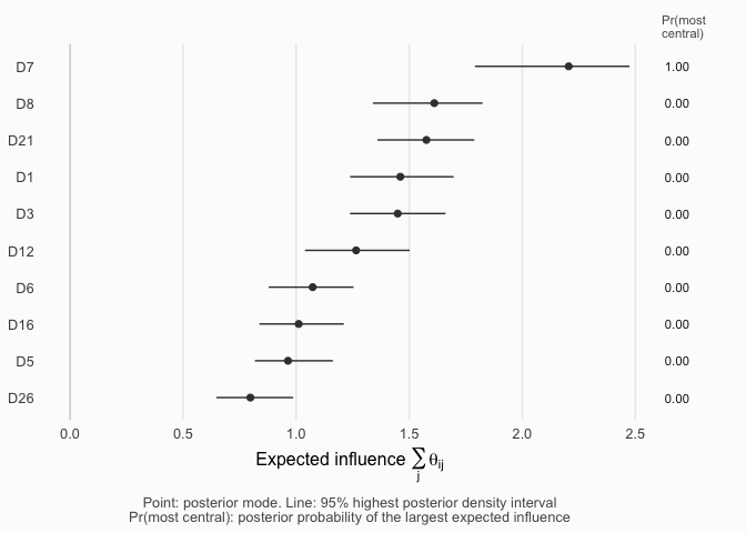

Expected influence of the 10 items with highest posterior density intervals and the posterior probability of being the most central item

plot of chunk centrality

Item D7 has the largest expected influence, and is the most central item in 100% of the posterior draws. For a dmrfit fit, plot(fit, type = "centrality") shows the estimates with Wald intervals.

Which method when

CoRe approximates the posterior based on the full likelihood. For small networks, this posterior can be sampled exactly, because its normalizing constant can be computed by enumerating all $(m + 1)^p$ response patterns. This gives a direct check of the approximation, here on the first five items ( $4^5 = 1{,}024$ response patterns):

five <- items[1:5]
fit_core <- dmrfit_bayes(rads2[, five], nsim = 5000, burnin = 1000, progress = FALSE)
fit_exact <- dmrfit_bayes(rads2[, five], method = "exact", nsim = 5000, burnin = 1000, progress = FALSE)
sd_ratio <- apply(fit_core$draws, 1, sd) / apply(fit_exact$draws, 1, sd)
summary(sd_ratio)
#>    Min. 1st Qu.  Median    Mean 3rd Qu.    Max. 
#>  0.9780  0.9972  1.0506  1.0485  1.0742  1.1646

The posterior standard deviations of CoRe are close to those of the exact posterior, and slightly larger on average (median ratio 1.05, largest 1.16). This agrees with the theory, because the GHW covariance is at least as large as the inverse Fisher information, with equality when the pseudo-likelihood is efficient, and the residual gap grows for small $n$ relative to the number of parameters (Arena and Marsman, 2026). The other options of dmrfit_bayes() are the following.

method = "core" (default): the coordinate-rescaled pseudo-posterior, as fast as sampling the pseudo-posterior.
method = "adacore": adapts the rescaling during burn-in, at the running mean of the draws.
method = "exact": the posterior based on the full likelihood, by enumeration, only for small networks (up to control$max_states response patterns).
method = "dmh": the posterior based on the full likelihood with the double Metropolis-Hastings algorithm (Liang, 2010), for any network size, but much slower: a reference rather than a routine choice.
scale, for method = "core": the covariance the pseudo-posterior is rescaled to, the GHW covariance ("ghw", default), or the inverse of a Monte Carlo estimate of the negative Hessian of the full log-posterior, at the pseudo-posterior mode ("mch") or at the Robbins-Monro estimate of the full-posterior mode ("rm"). The last two simulate data from the model and are slower.

References

Arena, G. and Marsman, M. (2026). Bayesian inference for discrete Markov random fields through coordinate rescaling. arXiv preprint. https://doi.org/10.48550/arXiv.2601.17205
Geys, H., Molenberghs, G., and Ryan, L. M. (1999). Pseudolikelihood modeling of multivariate outcomes in developmental toxicology. Journal of the American Statistical Association, 94(447), 734-745. https://doi.org/10.1080/01621459.1999.10474176
Liang, F. (2010). A double Metropolis-Hastings sampler for spatial models with intractable normalizing constants. Journal of Statistical Computation and Simulation, 80(9), 1007-1022.
Pace, L., Salvan, A., and Sartori, N. (2011). Adjusting composite likelihood ratio statistics. Statistica Sinica, 21(1), 129-148.
Ramos-Vera, C., Quispe Callo, G., Basauri Delgado, M., Vallejos Saldarriaga, J., and Saintila, J. (2023). Factorial and network structure of the Reynolds Adolescent Depression Scale (RADS-2) in Peruvian adolescents. PLOS ONE, 18(5), e0286081.
Robinaugh, D. J., Millner, A. J., and McNally, R. J. (2016). Identifying highly influential nodes in the complicated grief network. Journal of Abnormal Psychology, 125(6), 747-757.
Skare, Ø., Bølviken, E., and Holden, L. (2003). Improved sampling-importance resampling and reduced bias importance sampling. Scandinavian Journal of Statistics, 30(4), 719-737.
Titsias, M. K. (2024). Optimal preconditioning and Fisher adaptive Langevin sampling. In Proceedings of the 37th International Conference on Neural Information Processing Systems (NIPS ’23). Red Hook, NY, USA: Curran Associates.